Welcome to kafe, the Karlsruhe Fit Environment¶

kafe is a data fitting framework designed for use in undergraduate physics lab courses. It provides a basic Python toolkit for fitting models to data as well as visualisation of the data and the model function. It relies on Python packages such as numpy and matplotlib, and uses the Python interface to the minimizer Minuit contained in the data analysis framework ROOT or in the Python package iminuit.

kafe Overview¶

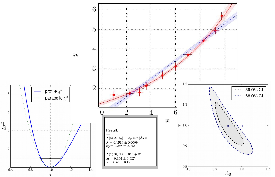
Graphical output generated with kafe.¶

The kafe package provides a rather general approach to fitting of a model function to two-dimensional data points with correlated uncertainties in both dimensions. The Python API guarantees full flexibility for data input. Helper functions for file-based input and some examples are available for own applications.

Applications range from performing a simple average of measurements to complex situations with both correlated (systematic) and uncorrelated (statistical) uncertainties on the measurements of the x and y values described by a non-linear model function depending on a large number of parameters.

The model function describes the y values as a function of the x-values and a set of model parameters {p}, y=f(x; {p}). Full flexibility exists as model functions are implemented as Python code. Again, examples are provided, but user implementations are supported as well.

Fitting is based on the χ²-method, assuming Gaussian errors and correlations described by covariance matrices. The level of agreement between data points and the fit model is expressed in terms of the χ² probability, i. e. the probability to find less agreement between data and model than actually observed. Full access to the covariance matrix of the - typically correlated - model parameters is provided.

The graphical output visualises the data and the fit model at the best-fit-point of the parameters and also shows the uncertainty of the fit model as a light band surrounding the line representing the model function. Plotting of confidence level contours for pairs of parameters or profiling of the χ² curves for each of the fit parameters are also provided.

Code Structure¶

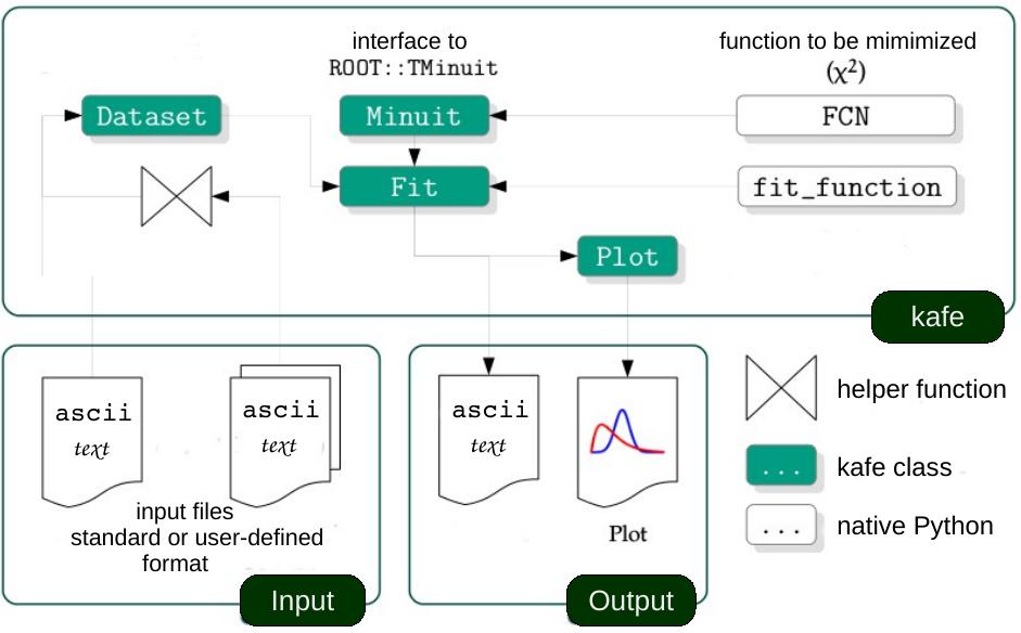
Code structure of the kafe package¶

The code of kafe is centred around very few classes to handle Data input, fitting and plotting, as illustrated in the figure on the right-hand side.

Data, their uncertainties, and, optionally, the correlations of the uncertainties - are passed through the interface of the kafe class Dataset. Input can be included in the Python code or is read from files in standardised or user-defined formats. The representation of the data within the Dataset class is minimalistic, consisting of the x and y values and the full covariance matrices of their uncertainties. Correlated errors between x and y values are not supported yet, as such use cases are rare.

A helper function, build_dataset(), is available to transform various error models, like a combination of independent and correlated errors or common absolute or relative errors, to this basic format.

Adding a model function, taken either from a prepared set of fit functions within kafe or from a user’s own Python implementation, results in a Fit object, which controls the minimizer Minuit. Access to the final results of the fitting procedure is provided by data members of the Fit class.

One or multiple fit objects, i. e. the input data and model functions(s) at the best-fit point in parameter-space, are visualised by the class Plot with the help of matplotlib functionality. The plot module also contains functionality to display the model uncertainty by surrounding the model function at the best-fit values of the parameters by a light band, the one-σ uncertainty band, which is obtained by propagation of the uncertainties of the fit parameters taking into account their correlations.

Two-dimensional contour lines of pairs of parameters are obtained with the method plot_contour() of the Fit class, which internally relies on the mncont method of the Minuit package. Contour curves are obtained from a scan of the χ²-function around a fixed value, where each point on the curve represents the minimum with respect to all other free parameters in the fit, thus taking into account the correlation of the considered pair of parameters with all other parameters of the model.

In a similar way, the method plot_profile() provides profiled χ² curves, i. e. the value of the minimal χ² as a function of one parameter while all other parameters are allowed to vary.

Fitting in a Nutshell¶

Fitting with kafe in a nutshell goes like this:

create a Dataset object from your measurement data:

>>> my_d = kafe.Dataset(data=[[0., 1., 2.], [1.23, 3.45, 5.62]])

add errors (uncertainties) to your Dataset:

>>> my_d.add_error_source('y', 'simple', 0.5)  # y errors, all +/- 0.5

import a model function from kafe.function_library (or define one yourself):
```
>>> from kafe.function_library import linear_2par
```
create a Fit object from your Dataset and your model function:
```
>>> my_f = kafe.Fit(my_d, linear_2par)
```
do the fit:
```
>>> my_f.do_fit()
```

(optional) if you want to see a plot of the result, use the Plot object:

>>> my_p = kafe.Plot(my_f)
>>> my_p.plot_all()
>>> my_p.show()

Example¶

Only very few lines of Python code are needed to perform fits with kafe. The snippet of code shown below performs a fit of a quadratic function to some data points with uncertainties:

from kafe import *
from kafe.function_library import quadratic_3par

#### build a Dataset instance:
myDataset = build_dataset(
    [0.05,0.36,0.68,0.80,1.09,1.46,1.71,1.83,2.44,2.09,3.72,4.36,4.60],
    [0.35,0.26,0.52,0.44,0.48,0.55,0.66,0.48,0.75,0.70,0.75,0.80,0.90],
    yabserr=[0.06,0.07,0.05,0.05,0.07,0.07,0.09,0.1,0.11,0.1,0.11,0.12,0.1],
    title='some data',
    axis_labels=['$x$', '$y=f(x)$'])

#### Create the Fit object
myFit = Fit(myDataset, quadratic_3par)
# Set initial values and error estimates
myFit.set_parameters((0., 1., 0.2), (0.5, 0.5, 0.5))
# Do the Fit
myFit.do_fit()

#### Create result plots and output them
myPlot = Plot(myFit)
myPlot.plot_all()
myPlot.save('kafe_example0.pdf') # to file

myPlot.show()                    # to screen

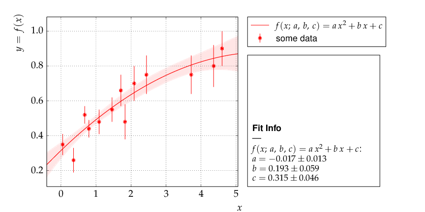
The output in text form (also available via various get_...() methods of the Fit class) contains the values of the parameters at the best-fit point, their correlation matrix and the fit probability. The example produces the following graphical output:

Example: Data points with one-dimensional error bars compared to a quadratic model function with kafe.¶

The parametrisation chosen in this example leads to a strong correlation of the fit parameters. This can be graphically visualised by adding the following lines at the end of the example:

### Create and save contour plots
contour1 = myFit.plot_contour(0, 1, dchi2=[1., 2.3])
contour2 = myFit.plot_contour(0, 2, dchi2=[1., 2.3])
contour3 = myFit.plot_contour(1, 2, dchi2=[1., 2.3])
contour1.savefig('kafe_example0_contour1.pdf')
contour2.savefig('kafe_example0_contour2.pdf')
contour3.savefig('kafe_example0_contour3.pdf')

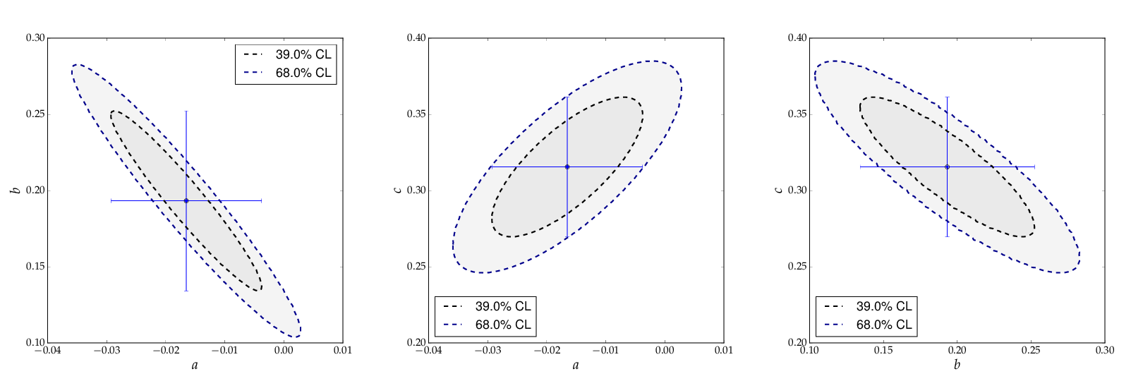
The example code produces two confidence-level contours for each pair of parameters (with id=0, id=1 and id=2), corresponding to an increase of the χ²-function with respect to the minimum by the values given in the list passed as the third parameter to the method myFit.plot_contour(). The resulting graphical representation, as shown below, displays the 39% contours, corresponding to the one-sigma errors, and the 68% contours. The uncertainties on each parameter, indicated by the error bars, are also shown. They correspond to the projections of the one-sigma contours on the axes.

Contour curves of a pairs of paramters a, b and c of the example above, calculated with kafe.¶

More and advanced examples - like fitting different models to one data set, comparison of different data sets with model functions, averaging of correlated measurements or fits with a large number of parameters - are provided as part of the kafe distribution and are described in the section Examples below. They may serve as a starting point for own applications.