Beginners Guide
This section covers the basics of using kafe2 for fitting parametric models to data by showing examples. Specifically, it teaches users how to specify measurement data and uncertainties, how to specify model functions, and how to extract the fit results.
An interactive Jupyter Notebook teaching the usage of kafe2 with Python is available in English and German.
More detailed information for the advanced use of kafe2 is found in the User Guide and in the API documentation.
Basic Fitting Procedure
Generally, any simple fit performed by kafe2 can be divided into the following steps:
Specifying the data
Specifying the uncertainties
Specifying the model function
Performing the fit
Extracting the fit results
This document will gradually introduce the above steps via example code.
Using kafe2go
Using kafe2go is the simplest way of performing a fit. Here all the necessary information and properties like data and uncertainties are specified in a YAML file (.yml file extension). To perform the fit, simply run:
kafe2go path/to/fit.yml
Using Python
When using kafe2 via a Python script it is possible to precisely control how fits are performed and plotted. For using kafe2 inside a Python script, import the required kafe2 modules:
from kafe2 import XYFit, Plot
If a code example contains a line similar to data = XYContainer.from_file("data.yml")
the corresponding YAML file can be found in the same directory that contains the example Python
script.
The example files can be found on
GitHub.
Example 1: Line Fit
The first example is the simplest use of a fitting framework: performing a line fit.
A linear function of the form 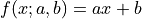 is made to align with
a series of xy data points that have some uncertainty along the x-axis
and the y-axis.
This example demonstrates how to perform such a line fit in kafe2 and
how to extract the results.
is made to align with
a series of xy data points that have some uncertainty along the x-axis
and the y-axis.
This example demonstrates how to perform such a line fit in kafe2 and
how to extract the results.
kafe2go
To run this example, open a text editor and save the following file contents
as a YAML file named line_fit.yml.
# Example 01: Line fit
# In this example a line f(x) = a * x + b is being fitted
# to some data points with pointwise uncertainties.

# The minimal keywords needed to perform a fit are x_data,
# y_data, and y_errors.
# You might also want to define x_errors.

# Data is defined by lists:
x_data: [1.0, 2.0, 3.0, 4.0]

# For errors lists describe pointwise uncertainties.
# By default the errors will be uncorrelated.
x_errors: [0.05, 0.10, 0.15, 0.20]

# Because x_errors is equal to 5% of x_data we could have also defined it like this:
# x_errors: 5%

# In total the following x data will be used for the fit:
# x_0: 1.0 +- 0.05
# x_1: 2.0 +- 0.10
# x_2: 3.0 +- 0.15
# x_3: 4.0 +- 0.20

# In yaml lists can also be written out like this:
y_data:
- 2.3
- 4.2
- 7.5
- 9.4

# The above is equivalent to
# y_data: [2.3, 4.2, 7.5, 9.4]

# For errors a single float gives each data point
# the same amount of uncertainty:
y_errors: 0.4

# The above is equivalent to
# y_errors: [0.4, 0.4, 0.4, 0.4]

# In total the following y data will be used for the fit:
# y_0: 2.3 +- 0.4
# y_1: 4.2 +- 0.4
# y_2: 7.5 +- 0.4
# y_3: 9.4 +- 0.4
Then open a terminal, navigate to the directory where the file is located and run
kafe2go line_fit.yml
Python
The same fit can also be performed by using a Python script.
python codeimport matplotlib.pyplot as plt
# Create an XYContainer object to hold the xy data for the fit.
xy_data = XYContainer(x_data=[1.0, 2.0, 3.0, 4.0],
y_data=[2.3, 4.2, 7.5, 9.4])
# x_data and y_data are combined depending on their order.
# The above translates to the points (1.0, 2.3), (2.0, 4.2), and (4.0, 9.4).
# Important: Specify uncertainties for the data.
xy_data.add_error(axis='x', err_val=0.1)
xy_data.add_error(axis='y', err_val=0.4)
# Create an XYFit object from the xy data container.
# By default, a linear function f=a*x+b will be used as the model function.
line_fit = Fit(data=xy_data)
# Perform the fit: Find values for a and b that minimize the
# difference between the model function and the data.
line_fit.do_fit() # This will throw an exception if no errors were specified.
# Optional: Print out a report on the fit results on the console.
line_fit.report()
# Optional: Create a plot of the fit results using Plot.
plot = Plot(fit_objects=line_fit) # Create a kafe2 plot object.
plot.plot() # Do the plot.
# Show the fit result.
plt.show()
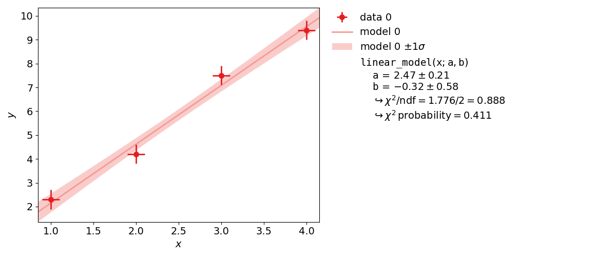
Example 2: Model Functions
In experimental physics a line fit will only suffice for a small number of applications. In most cases you will need a more complex model function with more parameters to accurately model physical reality. This example demonstrates how to specify arbitrary model functions for a kafe2 fit. When a different function has to be fitted, those functions need to be defined either in the YAML file or the Python script.
 has an expected value of 1, if both the model function and the error
estimates are correct.
When using the same dataset and error estimates a smaller value of
means a better fit.
Thus the exponential function describes the dataset more accurately than the line function.
has an expected value of 1, if both the model function and the error
estimates are correct.
When using the same dataset and error estimates a smaller value of
means a better fit.
Thus the exponential function describes the dataset more accurately than the line function.
An exponential function is a non-linear function!
Non-linear refers to the linearity of the parameters.
So any polynomial like  is a linear function of the parameters
 ,
,  and
and  .
So an exponential function
.
So an exponential function  is non-linear in its parameter
  .
Thus the profile of
.
Thus the profile of  can have a non-parabolic shape.
If that is the case, uncertainties of the form
can have a non-parabolic shape.
If that is the case, uncertainties of the form  won’t be accurate.
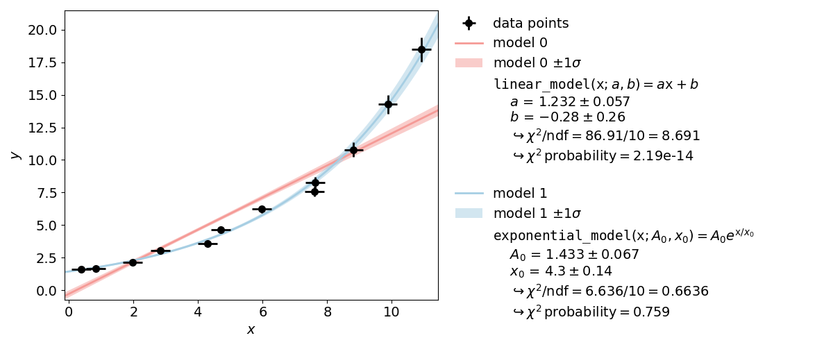
To see the shape of the profiles and contours, please create a contour plot of the fitted
parameters.
This can be done by appending the -c or --contours option to kafe2go.
Additionally a grid can be added to the contour plots with the --grid all flag.
To achieve the same with a Python script, import the ContoursProfiler with
from kafe2 import ContoursProfiler.
This class can create contour and profile plots.
The usage is shown in the following code example.
By creating the contours in a Python script the user can more precisely control the appearance of
the contour plot as well as which parameters to profile.
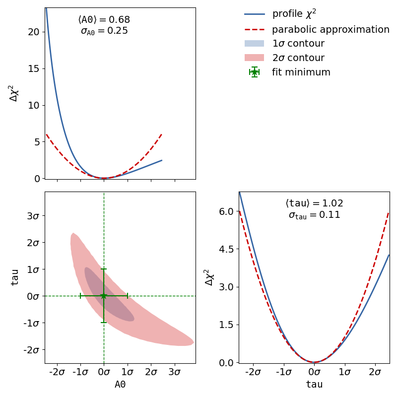
The corresponding contour plot for the exponential fit shown above looks like this:
When looking at the profiles of the parameters, the deformation is effectively not
present.
In this case the fit results and uncertainties are perfectly fine and are can be used as is.
If a profile has a non-parabolic shape, uncertainties of the form won’t be
accurate.
Please refer to Example 4: Non-Linear Fits for more information.
kafe2go
Inside a YAML file custom fit functions can be defined with the model_function keyword.
The custom function must be a Python function. NumPy functions are supported without extra import
statements, as shown in the example.
For more advanced fit functions, consider using kafe2 inside a Python script.
x_data:
- 0.3811286952593707
- 0.8386314422752791
- 1.965701211114396
- 2.823689293793774
- 4.283116179196964
- 4.697874987903564
- 5.971438461333021
- 7.608558039032569
- 7.629881032308029
- 8.818924700702548
- 9.873903963026425
- 10.913590565136278
x_errors:
- correlation_coefficient: 0.0
  error_value: 0.3  # use absolute errors, in this case always 0.3
  relative: false
  type: simple
y_data:
- 1.604521233331755
- 1.6660578688633165
- 2.1251504836493296
- 3.051883842283453
- 3.5790120649006685
- 4.654148130730669
- 6.213711922872129
- 7.576981533273081
- 8.274440603191387
- 10.795366227038528
- 14.272404187046607
- 18.48681513824193
y_errors:
- correlation_coefficient: 0.0
  error_value: 0.05
  relative: true  # use relative errors, in this case 5% of each value
  type: simple

model_function: |
  def exponential_model(x, A0=1., x0=5.):
      # Our second model is a simple exponential function
      # The kwargs in the function header specify parameter defaults.
      return A0 * np.exp(x/x0)
x_data:
- 0.3811286952593707
- 0.8386314422752791
- 1.965701211114396
- 2.823689293793774
- 4.283116179196964
- 4.697874987903564
- 5.971438461333021
- 7.608558039032569
- 7.629881032308029
- 8.818924700702548
- 9.873903963026425
- 10.913590565136278
x_errors:
- correlation_coefficient: 0.0
  error_value: 0.3  # use absolute errors, in this case always 0.3
  relative: false
  type: simple
y_data:
- 1.604521233331755
- 1.6660578688633165
- 2.1251504836493296
- 3.051883842283453
- 3.5790120649006685
- 4.654148130730669
- 6.213711922872129
- 7.576981533273081
- 8.274440603191387
- 10.795366227038528
- 14.272404187046607
- 18.48681513824193
y_errors:
- correlation_coefficient: 0.0
  error_value: 0.05
  relative: true  # use relative errors, in this case 5% of each value
  type: simple

model_function: |
  def linear_model(x, a, b):
      # Our first model is a simple linear function
      return a * x + b
To use multiple input files with kafe2go, simply run
kafe2go path/to/fit1.yml path/to/fit2.yml
To plot the fits in two separate figures append the --separate flag to the kafe2go command.
kafe2go path/to/fit1.yml path/to/fit2.yml --separate
For creating a contour plot, simply add -c to the command line. This will create contour plots
for all given fits.
kafe2go path/to/fit1.yml path/to/fit2.yml --separate -c
Python
Inside a Python script a custom function is defined like this:
# To define a model function for kafe2 simply write it as a python function
# Important: The model function must have the x among its arguments
def linear_model(x, a, b):
    # Our first model is a simple linear function
    return a * x + b

def exponential_model(x, A0=1., x0=5.):
    # Our second model is a simple exponential function
    # The kwargs in the function header specify parameter defaults.
    return A0 * np.exp(x/x0)
Those functions are passed on to the Fit objects:
# Create 2 Fit objects with the same data but with different model functions
linear_fit = Fit(data=xy_data, model_function=linear_model)
exponential_fit = Fit(data=xy_data, model_function=exponential_model)
It’s also possible to assign LaTeX expressions to the function and its variables.
# Optional: Assign LaTeX strings to parameters and model functions.
linear_fit.assign_parameter_latex_names(a='a', b='b')
linear_fit.assign_model_function_latex_expression("{a}{x} + {b}")
exponential_fit.assign_parameter_latex_names(A0='A_0', x0='x_0')
exponential_fit.assign_model_function_latex_expression("{A0} e^{{{x}/{x0}}}")
Please note that the function LaTeX expression needs to contain all parameters present in the function definition. The placeholders are then automatically replaced by their corresponding LaTeX names. Due to the way Python implements string formatting, curly braces used in LaTeX need to be typed twice, as shown in the code example.
The full example additionally contains the creation of a contour plot. The corresponding lines are highlighted in the following example.
python codefrom kafe2 import XYContainer, Fit, Plot, ContoursProfiler
import numpy as np
import matplotlib.pyplot as plt
# To define a model function for kafe2 simply write it as a python function
# Important: The model function must have the x among its arguments
def linear_model(x, a, b):
# Our first model is a simple linear function
return a * x + b
def exponential_model(x, A0=1., x0=5.):
# Our second model is a simple exponential function
# The kwargs in the function header specify parameter defaults.
return A0 * np.exp(x/x0)
# Read in the measurement data from a yaml file.
# For more information on reading/writing kafe2 objects from/to files see TODO
xy_data = XYContainer.from_file("data.yml")
# Create 2 Fit objects with the same data but with different model functions
linear_fit = Fit(data=xy_data, model_function=linear_model)
exponential_fit = Fit(data=xy_data, model_function=exponential_model)
# Optional: Assign LaTeX strings to parameters and model functions.
linear_fit.assign_parameter_latex_names(a='a', b='b')
linear_fit.assign_model_function_latex_expression("{a}{x} + {b}")
exponential_fit.assign_parameter_latex_names(A0='A_0', x0='x_0')
exponential_fit.assign_model_function_latex_expression("{A0} e^{{{x}/{x0}}}")
# Perform the fits.
linear_fit.do_fit()
exponential_fit.do_fit()
# Optional: Print out a report on the result of each fit.
linear_fit.report()
exponential_fit.report()
# Optional: Create a plot of the fit results using Plot.
p = Plot(fit_objects=[linear_fit, exponential_fit], separate_figures=False)
# Optional: Customize the plot appearance: only show the data points once.
p.customize('data', 'color', values=['k', 'none']) # hide points for second fit
p.customize('data', 'label', values=['data points', None]) # no second legend entry
# Do the plotting.
p.plot(fit_info=True)
# Optional: Create a contour plot for the exponential fit to show the parameter correlations.
cpf = ContoursProfiler(exponential_fit)
cpf.plot_profiles_contours_matrix(show_grid_for='contours')
# Show the fit results.
plt.show()
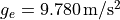
Example 3: Parameter Constraints
The models used to describe physical phenomena usually depend on a multitude of parameters. However, for many experiments only one of the parameters is of actual interest to the experimenter. Still, because model parameters are generally not uncorrelated the experimenter has to factor in the nuisance parameters for their estimation of the parameter of interest.
Historically this has been done by propagating the uncertainties of the nuisance parameters onto the y-axis of the data and then performing a fit with those uncertainties. Thanks to computers, however, this process can also be done numerically by applying parameter constraints. This example demonstrates the usage of those constraints in the kafe2 framework.
More specifically, this example will simulate the following experiment:
A steel ball of radius  has been connected to the ceiling by a string of length
  ,
forming a pendulum. Due to earth’s gravity providing a restoring force this system is a harmonic
oscillator. Because of friction between the steel ball and the surrounding air the oscillator is
also damped by the viscous damping coefficient .
,
forming a pendulum. Due to earth’s gravity providing a restoring force this system is a harmonic
oscillator. Because of friction between the steel ball and the surrounding air the oscillator is
also damped by the viscous damping coefficient .
The goal of the experiment is to determine the local strength of earth’s gravity  . Since
the earth is shaped like an ellipsoid the gravitational pull varies with latitude: it’s strongest
at the poles with
. Since
the earth is shaped like an ellipsoid the gravitational pull varies with latitude: it’s strongest
at the poles with 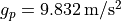 and it’s weakest at the equator with
 . For reference, at Germany’s latitude lies at
approximately
. For reference, at Germany’s latitude lies at
approximately  .
.
kafe2go
Parameter constraints are straightforward to use with kafe2go. After defining the model function parameter constraints can be set. Simple gaussian constraints can be defined with the parameter name followed by the required information as highlighted in the example. For more information on parameter constraints via a covariance matrix, please refer to Parameter Constraints.
constraints.ymlx_data: [0.0, 0.5, 1.0, 1.5, 2.0, 2.5, 3.0, 3.5, 4.0, 4.5, 5.0, 5.5, 6.0, 6.5, 7.0, 7.5, 8.0, 8.5,
9.0, 9.5, 10.0, 10.5, 11.0, 11.5, 12.0, 12.5, 13.0, 13.5, 14.0, 14.5, 15.0, 15.5, 16.0,
16.5, 17.0, 17.5, 18.0, 18.5, 19.0, 19.5, 20.0, 20.5, 21.0, 21.5, 22.0, 22.5, 23.0, 23.5,
24.0, 24.5, 25.0, 25.5, 26.0, 26.5, 27.0, 27.5, 28.0, 28.5, 29.0, 29.5, 30.0, 30.5, 31.0,
31.5, 32.0, 32.5, 33.0, 33.5, 34.0, 34.5, 35.0, 35.5, 36.0, 36.5, 37.0, 37.5, 38.0, 38.5,
39.0, 39.5, 40.0, 40.5, 41.0, 41.5, 42.0, 42.5, 43.0, 43.5, 44.0, 44.5, 45.0, 45.5, 46.0,
46.5, 47.0, 47.5, 48.0, 48.5, 49.0, 49.5, 50.0, 50.5, 51.0, 51.5, 52.0, 52.5, 53.0, 53.5,
54.0, 54.5, 55.0, 55.5, 56.0, 56.5, 57.0, 57.5, 58.0, 58.5, 59.0, 59.5, 60.0]
x_errors: 0.001
y_data: [0.6055317575993914, 0.5169107902610475, 0.3293169273559535, 0.06375859733814328,
-0.22640917641452488, -0.4558011426302008, -0.5741274235093591, -0.5581292464350779,
-0.4123919729458466, -0.16187396188197636, 0.11128294449725282, 0.3557032748758762,
0.5123991632742368, 0.5426212570679745, 0.441032201346871, 0.2530635717934812,
-0.018454841476861578, -0.27767282674995675, -0.4651897678670606, -0.5496969201663507,
-0.5039723480612176, -0.32491507193649194, -0.07545061334934718, 0.17868596924060803,
0.38816743920465974, 0.5307390166315159, 0.5195411750524918, 0.3922352276601664,
0.1743316249378316, -0.08489324112691513, -0.31307737388477896, -0.47061848549403956,
-0.5059137659253059, -0.4255733083473707, -0.24827692102709906, -0.013334081799533964,
0.21868390151118114, 0.40745363855032496, 0.4900638626421252, 0.4639947376885959,
0.3160179896333209, 0.11661884242058931, -0.15370888958327286, -0.32616191426973545,
-0.45856921225721586, -0.46439857887558106, -0.3685539265001533, -0.1830244989818371,
0.03835530881316253, 0.27636300051486506, 0.4163001580121898, 0.45791960756716926,
0.4133277046353799, 0.2454571744527809, 0.02843505139404641, -0.17995259849041545,
-0.3528170613993332, -0.4432670688586229, -0.4308872405896063, -0.3026153676925856,
-0.10460001285649327, 0.10576999137260902, 0.2794125634785019, 0.39727960494083775,
0.44012013094335295, 0.33665573392945614, 0.19241116925921273, -0.01373255454051425,
-0.2288093781464643, -0.36965277845455136, -0.4281953074871928, -0.3837254105792804,
-0.2439384794237307, -0.05945292033865969, 0.12714573185667402, 0.31127632080817996,
0.38957820781361946, 0.4022425989547513, 0.2852587536434507, 0.12097975879552739,
-0.06442727622110235, -0.25077071692351, -0.3414562050547135, -0.3844271968533089,
-0.3344326061358699, -0.1749451011511041, -0.016716872087832926, 0.18543436492361495,
0.322914548974734, 0.37225887677620817, 0.3396788239855797, 0.254332254048965,
0.0665429944525343, -0.11267963115652598, -0.2795347352658008, -0.37651751469292644,
-0.3654799155251143, -0.28854786660062454, -0.14328549945642755, 0.04213065692623846,
0.2201386996949766, 0.32591680654151617, 0.3421258708802321, 0.32458251078266503,
0.18777342536595865, 0.032971092778669095, -0.13521542014013244, -0.3024666212766573,
-0.34121930021830144, -0.33201664443451445, -0.21960116119767256, -0.07735846981040519,
0.09202435934084172, 0.24410808130924241, 0.3310159788871507, 0.34354629209994936,
0.2765230394100408, 0.12467034370454594, -0.012680322294530635, -0.1690136862958978,
-0.27753009059653394]
y_errors: 0.01
# Because the model function is oscillating the fit needs to be initialized with near guesses for
# unconstrained parameters in order to converge.
# To use starting values for the fit, specify them as default values in the fit function.
model_function: |
def damped_harmonic_oscillator(x, y_0=1.0, l=1.0, r=1.0, g=9.81, c=0.01):
# Model function for a pendulum as a 1d, damped harmonic oscillator with zero initial speed
# x = time, y_0 = initial_amplitude, l = length of the string,
# r = radius of the steel ball, g = gravitational acceleration, c = damping coefficient
# effective length of the pendulum = length of the string + radius of the steel ball
l_total = l + r
omega_0 = np.sqrt(g / l_total) # phase speed of an undamped pendulum
omega_d = np.sqrt(omega_0 ** 2 - c ** 2) # phase speed of a damped pendulum
return y_0 * np.exp(-c * x) * (np.cos(omega_d *x) + c / omega_d * np.sin(omega_d * x))
parameter_constraints: # add parameter constraints
l:
value: 10.0
uncertainty: 0.001 # l = 10.0+-0.001
r:
value: 0.052
uncertainty: 0.001 # r = 0.052+-0.001
y_0:
value: 0.6
uncertainty: 0.006
relative: true # Make constraint uncertainty relative to value, y_0 = 0.6+-0.6%
Python
Using kafe2 inside a Python script, parameter constraints can be set with
fit.add_parameter_constraint(). The according section is highlighted in the code example below.
import numpy as np
import matplotlib.pyplot as plt

from kafe2 import XYContainer, Fit, Plot

# Relevant physical magnitudes and their uncertainties
l, delta_l = 10.0, 0.001  # length of the string, l = 10.0+-0.001 m
r, delta_r = 0.052, 0.001  # radius of the steel ball, r = 0.052+-0.001 kg
# amplitude of the steel ball at x=0 in degrees, y_0 = 0.6+-0.006% degrees
y_0, delta_y_0 = 0.6, 0.01  # Note that the uncertainty on y_0 is relative to y_0


# Model function for a pendulum as a 1d, damped harmonic oscillator with zero initial speed
# x = time, y_0 = initial_amplitude, l = length of the string,
# r = radius of the steel ball, g = gravitational acceleration, c = damping coefficient
def damped_harmonic_oscillator(x, y_0, l, r, g, c):
    # effective length of the pendulum = length of the string + radius of the steel ball
    l_total = l + r
    omega_0 = np.sqrt(g / l_total)  # phase speed of an undamped pendulum
    omega_d = np.sqrt(omega_0 ** 2 - c ** 2)  # phase speed of a damped pendulum
    return y_0 * np.exp(-c * x) * (np.cos(omega_d * x) + c / omega_d * np.sin(omega_d * x))


# Load data from yaml, contains data and errors
data = XYContainer.from_file(filename='data.yml')

# Create fit object from data and model function
fit = Fit(data=data, model_function=damped_harmonic_oscillator)

# Constrain model parameters to measurements
fit.add_parameter_constraint(name='l',   value=l,   uncertainty=delta_l)
fit.add_parameter_constraint(name='r',   value=r,   uncertainty=delta_r)
fit.add_parameter_constraint(name='y_0', value=y_0, uncertainty=delta_y_0, relative=True)

# Because the model function is oscillating the fit needs to be initialized with near guesses for
# unconstrained parameters in order to converge
g_initial = 9.81  # initial guess for g
c_initial = 0.01  # initial guess for c
fit.set_parameter_values(g=g_initial, c=c_initial)

# Optional: Set the initial values of the remaining parameters to correspond to their constraint
# values (this may help some minimization algorithms converge)
fit.set_parameter_values(y_0=y_0, l=l, r=r)

# Perform the fit
fit.do_fit()

# Optional: Print out a report on the fit results on the console.
fit.report()

# Optional: plot the fit results
plot = Plot(fit)
plot.plot(fit_info=True)

plt.show()
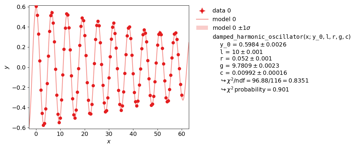
Example 4: Non-Linear Fits
Very often, when the fit model is a non-linear function of the parameters, the
function is not parabolic around the minimum.
A very common example of such a case is an exponential function
parametrized as shown in this example.
In the case of a non-linear fit, the minimum of a cost function is no longer shaped
like a parabola (with a model parameter on the x axis and on the y axis).
Now, you might be wondering why you should care about the shape of the function.
The reason why it’s important is that the common notation of  for fit results
is only valid for a parabola-shaped cost function.
If the function is distorted it will also affect your fit results!
for fit results
is only valid for a parabola-shaped cost function.
If the function is distorted it will also affect your fit results!
Luckily non-linear fits oftentimes still produce meaningful fit results as long as the distortion is
not too big - you just need to be more careful during the evaluation of your fit results.
A common approach for handling non-linearity is to trace the profile of the cost function (in this
case ) in either direction of the cost function minimum and find the points at which
the cost function value has increased by a specified amount relative to the cost function minimum.
In other words, two cuts are made on either side of the cost function minimum at a specified
height.
The two points found with this approach span a confidence interval for the fit parameter around the
cost function minimum.
The confidence level of the interval depends on how high you set the cuts for the cost increase
relative to the cost function minimum.
The one sigma interval described by conventional parameter errors is achieved by a cut at the fit
minimum plus  and has a confidence level of about 68%.
The two sigma interval is achieved by a cut at the fit minimum plus
and has a confidence level of about 68%.
The two sigma interval is achieved by a cut at the fit minimum plus  and has a
confidence level of about 95%, and so on.
The one sigma interval is commonly described by what is called asymmetric errors:
the interval limits are described relative to the cost function minimum as
and has a
confidence level of about 95%, and so on.
The one sigma interval is commonly described by what is called asymmetric errors:
the interval limits are described relative to the cost function minimum as
 .
.
In addition to non-linear function, the usage of x data errors leads to a non-linear fits as well.
kafe2 fits support the addition of x data errors - in fact we’ve been using them since the very
first example.
To take them into account the x errors are converted to y errors via multiplication with the
derivative of the model function.
In other words, kafe2 fits extrapolate the derivative of the model function at the x data values
and calculate how a difference in the x direction would translate to the y direction.
Unfortunately this approach is not perfect though.
Since we’re extrapolating the derivative at the x data values, we will only receive valid results
if the derivative doesn’t change too much at the scale of the x error.
Also, since the effective y error has now become dependent on the derivative of the model function
it will vary depending on our choice of model parameters.
This distorts our likelihood function - the minimum of a cost function will no
longer be shaped like a parabola (with a model parameter on the x axis and on the
y axis).
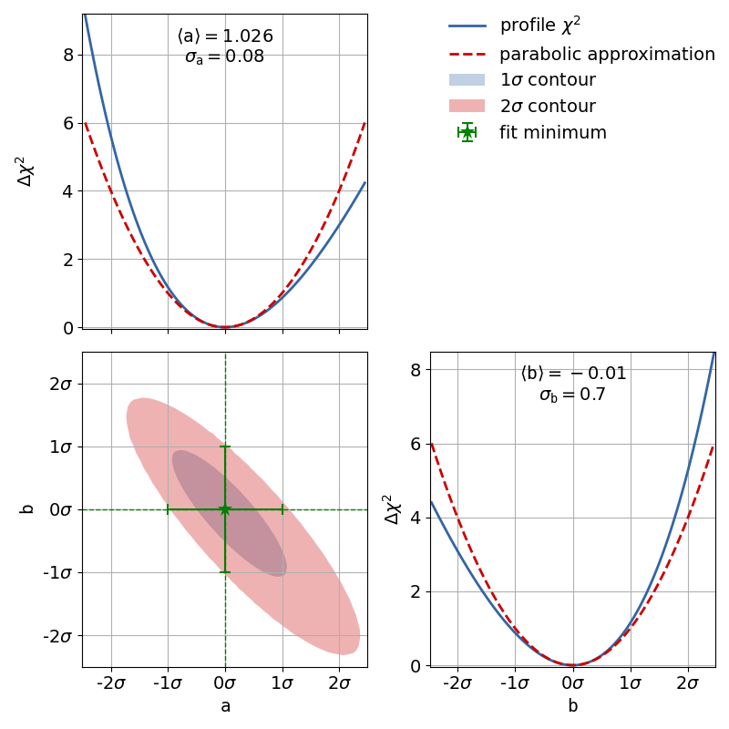
To demonstrate this, the second file x_errors will perform a line fit with much bigger
uncertainties on the x axis than on the y axis. The non-parabolic shape can be seen in the
one-dimensional profile scans.
kafe2go
To display asymmetric parameter uncertainties use the flag -a. In addition the profiles and
contours can be shown by using the -c flag. In the Python example a ratio between the data
and model function is shown below the plot. This can be done by appending the -r flag to
kafe2go.
# This is an example for a non-linear fit
# Please run with 'kafe2go -a -c' to show asymmetric uncertainties and the contour profiles

x_data: [0.8018943, 1.839664, 1.941974, 1.276013, 2.839654, 3.488302, 3.775855, 4.555187, 4.477186, 5.376026]
x_errors: 0.3
y_data: [0.2650644, 0.1472682, 0.08077234, 0.1850181, 0.05326301, 0.01984233, 0.01866309, 0.01230001, 0.009694612,
         0.002412357]
y_errors: [0.1060258, 0.05890727, 0.03230893, 0.07400725, 0.0213052, 0.00793693, 0.007465238, 0.004920005, 0.003877845,
           0.0009649427]

model_function: |
  def exponential(x, A0=1, tau=1):
      return A0 * np.exp(-x/tau)
The dataset used to show that big uncertainties on the x axis can cause the fit to be non-linear
follows here.
Keep in mind that kafe2go will perform a line fit if no fit function has been specified.
In order do add a grid to the contours, run kafe2go with the --grid all flag.
So to plot with asymmetric errors, the profiles and contour as well as a grid run
kafe2go x_errors.yml -a -c --grid all
# kafe2 XYContainer yaml representation written by johannes on 23.07.2019, 16:57.
type: xy
x_data:
- 0.0
- 1.0
- 2.0
- 3.0
- 4.0
- 5.0
- 6.0
- 7.0
- 8.0
- 9.0
- 10.0
- 11.0
- 12.0
- 13.0
- 14.0
- 15.0
y_data:
- 0.2991126116324785
- 2.558050235697161
- 1.2863728164289798
- 3.824686039107114
- 2.843373362329926
- 5.461953737679532
- 6.103072604470123
- 8.166562633164254
- 8.78250807001851
- 8.311966900704014
- 8.980727588512268
- 11.144142620167695
- 11.891326143534158
- 12.126133797209802
- 15.805993018808897
- 15.3488445186788
# The x errors are much bigger than the y errors. This will strongly distort the likelihood function.
x_errors: 1.0
y_errors: 0.1
Python
The relevant lines to display asymmetric uncertainties and to create the contour plot are highlighted in the code example below.
non_linear_fit.pyimport numpy as np
import matplotlib.pyplot as plt
from kafe2 import Fit, Plot, ContoursProfiler
def exponential(x, A0=1, tau=1):
return A0 * np.exp(-x/tau)
# define the data as simple Python lists
x = [8.018943e-01, 1.839664e+00, 1.941974e+00, 1.276013e+00, 2.839654e+00, 3.488302e+00, 3.775855e+00, 4.555187e+00,
4.477186e+00, 5.376026e+00]
xerr = 3.000000e-01
y = [2.650644e-01, 1.472682e-01, 8.077234e-02, 1.850181e-01, 5.326301e-02, 1.984233e-02, 1.866309e-02, 1.230001e-02,
9.694612e-03, 2.412357e-03]
yerr = [1.060258e-01, 5.890727e-02, 3.230893e-02, 7.400725e-02, 2.130520e-02, 7.936930e-03, 7.465238e-03, 4.920005e-03,
3.877845e-03, 9.649427e-04]
# create a fit object from the data arrays
fit = Fit(data=[x, y], model_function=exponential)
fit.add_error(axis='x', err_val=xerr) # add the x-error to the fit
fit.add_error(axis='y', err_val=yerr) # add the y-errors to the fit
fit.do_fit() # perform the fit
fit.report(asymmetric_parameter_errors=True) # print a report with asymmetric uncertainties
# Optional: create a plot
plot = Plot(fit)
plot.plot(asymmetric_parameter_errors=True, ratio=True) # add the ratio data/function and asymmetric errors
# Optional: create the contours profiler
cpf = ContoursProfiler(fit)
cpf.plot_profiles_contours_matrix() # plot the contour profile matrix for all parameters
plt.show()
The example to show that uncertainties on the x axis can cause a non-linear fit uses the YAML dataset given in the kafe2go section.
non_linear_fit.pyimport matplotlib.pyplot as plt
from kafe2 import XYContainer, Fit, Plot
from kafe2.fit.tools import ContoursProfiler
# Construct a fit with data loaded from a yaml file. The model function is the default of f(x) = a * x + b
nonlinear_fit = Fit(data=XYContainer.from_file('x_errors.yml'))
# The x errors are much bigger than the y errors. This will cause a distortion of the likelihood function.
nonlinear_fit.add_error('x', 1.0)
nonlinear_fit.add_error('y', 0.1)
# Perform the fit.
nonlinear_fit.do_fit()
# Optional: Print out a report on the fit results on the console.
# Note the asymmetric_parameter_errors flag
nonlinear_fit.report(asymmetric_parameter_errors=True)
# Optional: Create a plot of the fit results using Plot.
# Note the asymmetric_parameter_errors flag
plot = Plot(nonlinear_fit)
plot.plot(fit_info=True, asymmetric_parameter_errors=True)
# Optional: Calculate a detailed representation of the profile likelihood
# Note how the actual chi2 profile differs from the parabolic approximation that you would expect with a linear fit.
profiler = ContoursProfiler(nonlinear_fit)
profiler.plot_profiles_contours_matrix(show_grid_for='all')
plt.show()
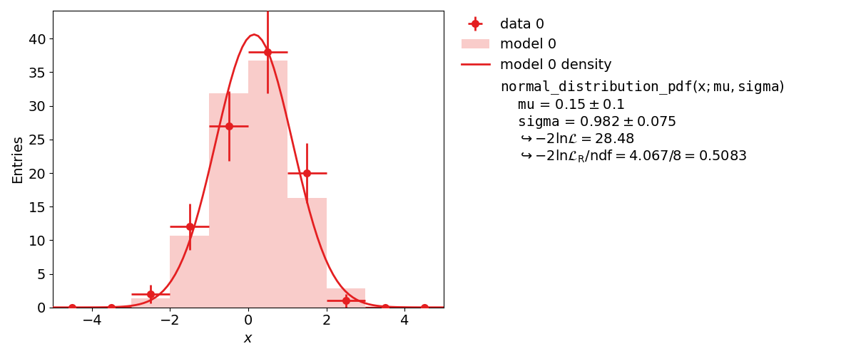
Example 5: Histogram Fit
In addition to the xy fits shown above kafe2 can also perform fits on one-dimensional datasets by binning the data. The distribution of a random stochastic variable follows a probability density function. This density needs to be normalized. The fit will determine the parameters of that density function, which the dataset is most likely to follow. If the given function is not normalized, please make sure to add an independent scale factor. The hist fit will try to normalize the function to one for the bin range. To get to the height of a bin, please multiply the results of the fitted function with the amount of entries N of the histogram.
kafe2go
In order to tell kafe2go that a fit is a histogram fit type: histogram has to specified
inside the YAML file.
type: histogram
n_bins: 10
bin_range: [-5, 5]
# alternatively an array for the bin edges can be specified
# bin_edges: [-5.0, -4.0, -3.0, -2.0, -1.0, 0.0, 1.0, 2.0, 3.0, 4.0, 5.0]
raw_data: [-2.7055035067034487, -2.2333305188904347, -1.7435697505734427, -1.6642777356357366,
           -1.5679848184835399, -1.3804124186290108, -1.3795713509086, -1.3574661967681951,
           -1.2985520413566647, -1.2520621390613085, -1.1278660506506273, -1.1072596181584253,
           -1.0450542861845105, -0.9892894612864382, -0.9094385163243246, -0.7867219919905643,
           -0.7852735587423539, -0.7735126880952405, -0.6845244856096362, -0.6703508433626327,
           -0.6675916809443503, -0.6566373185397965, -0.5958545249606959, -0.5845389846486857,
           -0.5835331341085711, -0.5281866305050138, -0.5200579414945709, -0.48433400194685733,
           -0.4830779584087414, -0.4810505389213239, -0.43133946043584287, -0.42594442622513157,
           -0.31654403621747557, -0.3001580802272723, -0.2517534764243999, -0.23262171181200844,
           -0.12253717030390852, -0.10096229375978451, -0.09647228959040793, -0.09569644689333284,
           -0.08737474828114752, -0.03702037295350094, -0.01793164577601821, 0.010882324251760892,
           0.02763866634172083, 0.03152268199512073, 0.08347307807870571, 0.08372272370359508,
           0.11250694814984155, 0.11309723105291797, 0.12917440700460459, 0.19490542653497123,
           0.22821618079608103, 0.2524597237143017, 0.2529456172163689, 0.35191851476845365,
           0.3648457146544489, 0.40123846238388744, 0.4100144162294351, 0.44475132818005764,
           0.48371376223538787, 0.4900044970651449, 0.5068133677441506, 0.6009580844076079,
           0.6203740420045862, 0.6221661108241587, 0.6447187743943843, 0.7332139482413045,
           0.7347787168653869, 0.7623603460722045, 0.7632360142894643, 0.7632457205433638,
           0.8088938754947214, 0.817906674531189, 0.8745869551496841, 0.9310849201186593,
           1.0060465798362423, 1.059538506895515, 1.1222643456638215, 1.1645916062658435,
           1.2108747344743727, 1.21215950663896, 1.243754543112755, 1.2521725699532695,
           1.2742444530825068, 1.2747154562887673, 1.2978477018565724, 1.304709072578339,
           1.3228758386699584, 1.3992737494003136, 1.4189560403246424, 1.4920066960096854,
           1.5729404508236828, 1.5805518556565201, 1.6857079988218313, 1.726087558454503,
           1.7511987724150104, 1.8289480135723097, 1.8602081565623672, 2.330215727183154]

model_density_function:
  model_function_formatter:
    latex_name: 'pdf'
    latex_expression_string: "\\exp{{\\frac{{1}}{{2}}(\\frac{{{x}-{mu}}}{{{sigma}}})^2}} /
    \\sqrt{{2\\pi{sigma}^2}}"
    arg_formatters:
      x: '{\tt x}'
      mu: '\mu'
      sigma: '\sigma'
  python_code: |
    def normal_distribution_pdf(x, mu, sigma):
        return np.exp(-0.5 * ((x - mu) / sigma) ** 2) / np.sqrt(2.0 * np.pi * sigma ** 2)
Python
To use a histogram fit in a Python script, just import it with
from kafe2 import HistContainer, HistFit.
The creation a a histogram requires the user to set the limits of the histogram and the amount of bins. Alternatively the bin edges for each bin can be set manually.
histogram_fit.pyimport numpy as np
import matplotlib.pyplot as plt
from kafe2 import HistContainer, Fit, Plot
def normal_distribution_pdf(x, mu, sigma):
return np.exp(-0.5 * ((x - mu) / sigma) ** 2) / np.sqrt(2.0 * np.pi * sigma ** 2)
# random dataset of 100 random values, following a normal distribution with mu=0 and sigma=1
data = np.random.normal(loc=0, scale=1, size=100)
# Create a histogram from the dataset by specifying the bin range and the amount of bins.
# Alternatively the bin edges can be set.
histogram = HistContainer(n_bins=10, bin_range=(-5, 5), fill_data=data)
# create the Fit object by specifying a density function
fit = Fit(data=histogram, model_function=normal_distribution_pdf)
fit.do_fit() # do the fit
fit.report() # Optional: print a report to the terminal
# Optional: create a plot and show it
plot = Plot(fit)
plot.plot()
plt.show()
Example 6: Unbinned Fit
An unbinned fit is needed when there are too few data points to create a (good) histogram. If a histogram is created from too few data points information can be lost or even changed by changing the exact value of one data point to the range of a bin. With an unbinned likelihood fit it’s still possible to fit the probability density function to the data points, as the likelihood of each data point is fitted.
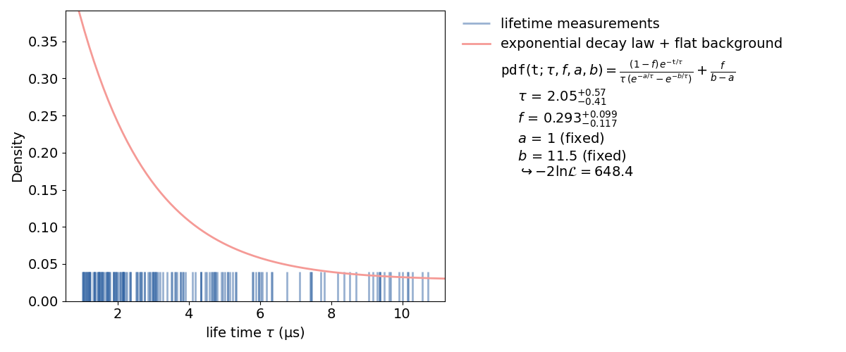
Inside a kafe2 fit, single parameters can be fixed as seen in the plot. When fixing a parameter, there must be a good reason to do so. In this case it’s the normalization of the probability distribution function. This, of course, could have been done inside the function itself. But if the user wants to change to normalization without touching the distribution function, this is a better way.
kafe2go
Similar to histogram fits, unbinned fits are defined by type: unbinned inside the YAML file.
How to fix single parameters is highlighted in the example below, as well as limiting the
background fbg to physically correct values.
type: unbinned
data: [7.420, 3.773, 5.968, 4.924, 1.468, 4.664, 1.745, 2.144, 3.836, 3.132, 1.568, 2.352, 2.132,
       9.381, 1.484, 1.181, 5.004, 3.060, 4.582, 2.076, 1.880, 1.337, 3.092, 2.265, 1.208, 2.753,
       4.457, 3.499, 8.192, 5.101, 1.572, 5.152, 4.181, 3.520, 1.344, 10.29, 1.152, 2.348, 2.228,
       2.172, 7.448, 1.108, 4.344, 2.042, 5.088, 1.020, 1.051, 1.987, 1.935, 3.773, 4.092, 1.628,
       1.688, 4.502, 4.687, 6.755, 2.560, 1.208, 2.649, 1.012, 1.730, 2.164, 1.728, 4.646, 2.916,
       1.101, 2.540, 1.020, 1.176, 4.716, 9.671, 1.692, 9.292, 10.72, 2.164, 2.084, 2.616, 1.584,
       5.236, 3.663, 3.624, 1.051, 1.544, 1.496, 1.883, 1.920, 5.968, 5.890, 2.896, 2.760, 1.475,
       2.644, 3.600, 5.324, 8.361, 3.052, 7.703, 3.830, 1.444, 1.343, 4.736, 8.700, 6.192, 5.796,
       1.400, 3.392, 7.808, 6.344, 1.884, 2.332, 1.760, 4.344, 2.988, 7.440, 5.804, 9.500, 9.904,
       3.196, 3.012, 6.056, 6.328, 9.064, 3.068, 9.352, 1.936, 1.080, 1.984, 1.792, 9.384, 10.15,
       4.756, 1.520, 3.912, 1.712, 10.57, 5.304, 2.968, 9.632, 7.116, 1.212, 8.532, 3.000, 4.792,
       2.512, 1.352, 2.168, 4.344, 1.316, 1.468, 1.152, 6.024, 3.272, 4.960, 10.16, 2.140, 2.856,
       10.01, 1.232, 2.668, 9.176]
label: "lifetime measurements"
x_label: "life time $\\tau$ (µs)"
y_label: "Density"
model_function:
  name: pdf
  latex_name: '{\tt pdf}'
  python_code: |
    def pdf(t, tau=2.2, fbg=0.1, a=1., b=9.75):
        """Probability density function for the decay time of a myon using the
        Kamiokanne-Experiment. The pdf is normed for the interval (a, b).
        :param t: decay time
        :param fbg: background
        :param tau: expected mean of the decay time
        :param a: the minimum decay time which can be measured
        :param b: the maximum decay time which can be measured
        :return: probability for decay time x"""
        pdf1 = np.exp(-t / tau) / tau / (np.exp(-a / tau) - np.exp(-b / tau))
        pdf2 = 1. / (b - a)
        return (1 - fbg) * pdf1 + fbg * pdf2
  arg_formatters:
    t: '{\tt t}'
    tau: '{\tau}'
    fbg: '{f}'
    a: '{a}'
    b: '{b}'
  latex_expression_string: "\\frac{{ (1-{fbg}) \\, e^{{ -{t}/{tau} }} }}
    {{ {tau} \\, (e^{{ -{a}/{tau} }} - e^{{ -{b}/{tau} }}) }} + \\frac{{ {fbg} }} {{ {b}-{a} }}"
model_label: "exponential decay law + flat background"
fixed_parameters:
  a: 1
  b: 11.5
limited_parameters:
  fbg: [0.0, 1.0]
Python
The fitting procedure is similar to the one of a histogram fit. How to fix single parameters is highlighted in the example below.
unbinned.pyfrom kafe2.fit import UnbinnedContainer, Fit, Plot
from kafe2.fit.tools import ContoursProfiler
import numpy as np
import matplotlib.pyplot as plt
def pdf(t, tau=2.2, fbg=0.1, a=1., b=9.75):
"""
Probability density function for the decay time of a myon using the Kamiokanne-Experiment.
The pdf is normed for the interval (a, b).
:param t: decay time
:param fbg: background
:param tau: expected mean of the decay time
:param a: the minimum decay time which can be measured
:param b: the maximum decay time which can be measured
:return: probability for decay time x
"""
pdf1 = np.exp(-t / tau) / tau / (np.exp(-a / tau) - np.exp(-b / tau))
pdf2 = 1. / (b - a)
return (1 - fbg) * pdf1 + fbg * pdf2
# load the data from the experiment
infile = "tau_mu.dat"
dT = np.loadtxt(infile)
data = UnbinnedContainer(dT) # create the kafe data object
data.label = 'lifetime measurements'
data.axis_labels = ['life time $\\tau$ (µs)', 'Density']
# create the fit object and set the pdf for the fit
fit = Fit(data=data, model_function=pdf)
# Fix the parameters a and b.
# Those are responsible for the normalization of the pdf for the range (a, b).
fit.fix_parameter("a", 1)
fit.fix_parameter("b", 11.5)
# constrain parameter fbg to avoid unphysical region
fit.limit_parameter("fbg", 0., 1.)
# assign latex names for the parameters for nicer display
fit.model_label = "exponential decay law + flat background"
fit.assign_parameter_latex_names(tau=r'\tau', fbg='f', a='a', b='b')
# assign a latex expression for the fit function for nicer display
fit.assign_model_function_latex_expression("\\frac{{ (1-{fbg}) \\, e^{{-{t}/{tau}}} }}"
"{{{tau} \\, (e^{{-{a}/{tau}}}-e^{{-{b}/{tau}}}) }}"
"+ \\frac{{ {fbg}}} {{{b}-{a}}}")
fit.do_fit() # perform the fit
fit.report(asymmetric_parameter_errors=True) # print a fit report to the terminal
plot = Plot(fit) # create a plot object
plot.plot(fit_info=True, asymmetric_parameter_errors=True) # plot the data and the fit
# Optional: create a contours profile
cpf = ContoursProfiler(fit, profile_subtract_min=False)
# Optional: plot the contour matrix for tau and fbg
cpf.plot_profiles_contours_matrix(parameters=['tau', 'fbg'])
plt.show() # show the plot(s)