Theoretical Foundation¶

This section briefly covers the underlying theoretical concepts upon which parameter estimation – and by extension kafe2 – is based.

Measurements and theoretical models¶

When measuring observable quantities, the results typically consist of a series of numeric measurement values: the data. Since no measurement is perfect, the data will be subject to measurement uncertainties. These uncertainties, also known as errors, are unavoidable and can be divided into two subtypes:

Independent uncertainties, as the name implies, affect each measurement independently: there is no relationship between the uncertainties of any two individual data points. Independent uncertainties are frequently caused by random fluctuations in the measurement values, either because of technical limitations of the experimental setup (electronic noise, mechanical vibrations) or because of the intrinsic statistical nature of the measured observable (as is typical in quantum mechanics, e. g. radioactive decays).

Correlated uncertainties arise due to effects that distort multiple measurements in the same way. Such uncertainties can for example be caused by a random imperfection of the measurement device which affects all measurements in the same way. The uncertainties of the measurements taken with such a device are no longer uncorrelated, but instead have one common uncertainty.

Historically uncertainties have been divided into statistical and systematic uncertainties. While this is appropriate when propagating the uncertainties of the input variables by hand it is not a suitable distinction for a numerical fit. In kafe2 multiple uncertainties are combined to construct a so-called covariance matrix. This is a matrix with the pointwise data variances on its diagonal and the covariances between two data points outside the diagonal. By using this covariance matrix for our fit we can estimate the uncertainty of our model parameters numerically with no need for propagating uncertainties by hand.

Parameter estimation¶

In parameter estimation, the main goal is to obtain best estimates for the parameters of a theoretical model by comparing the model predictions to experimental measurements.

This is typically done systematically by defining a quantity which expresses how well the model predictions fit the available data. This quantity is commonly called the loss function, or the cost function (the term used in kafe2 ). A statistical interpretation is possible if the cost function is related to the likelihood of the data with respect to a given model. In many cases the method of least squares is used, which is a special case of a likelihood for gaussian uncertainties.

The value of a cost function depends on the measurement data, the model function (often derived as a prediction from an underlying hypothesis or theory), and the uncertainties of the measurements and, possibly, the model. Cost functions are designed in such a way that the agreement between the measurements $d_i$ and the corresponding predictions $m_i$ provided by the model is best when the cost function reaches its global minimum.

For a given experiment the data $\bm{d}$ and the parametric form of the model $\bm{m}$ describing the data are constant. This means that the cost function $C$ then only depends on the model parameters, denoted here as a vector $\bm{p}$ in parameter space.

$C = C\left(\bm{d}, \bm{m}(\bm{p})\right) = C(\bm{p})$

Therefore parameter estimation essentially boils down to finding the vector of model parameters $\hat{\bm{p}}$ for which the cost function $C(\bm{p})$ is at its global minimum. In general this is a multidimensional optimization problem which is typically solved numerically. There are several algorithms and tools that can be used for this task: In kafe2 the Python package scipy can be used to minimize cost functions via its scipy.optimize module. Alternatively, kafe2 can use the MINUIT implementations TMinuit or iminuit when they are installed. More information on how to use the minimizers can be found in the User Guide.

Choosing a cost function¶

There are many cost functions used in statistics for estimating parameters. In physics experiments two are of particular importance: the sum of residuals and the negative logarithm of the likelihood, which are used in the least squares or the maximum likelihood methods, respectively. Incidentally, these are also the two basic types of cost functions that have been implemented in kafe2.

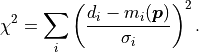
Least-squares (“chi-squared”)¶

The method of least squares is the standard approach in parameter estimation. To calculate the value of this cost function the differences between model and data are squared, then their sum is minimized with respect to the parameters (hence the name ‘least squares’). More formally, using the data covariance matrix $V$ , the cost function is expressed as follows:

$\chi^2(\bm{p}) = (\bm{d} - \bm{m}(\bm{p}))^T \ V^{-1} \ (\bm{d} - \bm{m}(\bm{p})).$

Since the value of the cost function at the minimum follows a $\chi^2$ distribution, and therefore the method of least squares is also known as chi-squared method. If the uncertainties of the data vector $\bm{d}$ are uncorrelated, all elements of $V$ except for its diagonal elements $\sigma_i^2$ (the squares of the $i$ -th point-wise measurement uncertainties) vanish.

The above formula then simply becomes

$\chi^2 = \sum_i \left( \frac{d_i - m_i(\bm{p})}{\sigma_i} \right)^2.$

All that is needed in this simple case is to divide the difference between data $d_i$ and model $m_i$ by the corresponding uncertainty $\sigma_i$ .

Computation-wise there is no noticeable difference for small datasets ( $O(100)$ data points). For very large datasets, however, the inversion of the full covariance matrix takes significantly longer than simply dividing by the point-wise uncertainties.

Negative log-likelihood¶

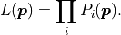
The method of maximum likelihood attempts to find the best estimation for the model parameters $\bm{p}$ by maximizing the probability with which such model parameters (under the given uncertainties) would result in the observed data $\bm{d}$ . More formally, the method of maximum likelihood searches for those values of $\bm{p}$ for which the so-called likelihood function of the parameters (likelihood for short) reaches its global maximum.

Using the probability of making a certain measurement given some values of model parameters $P(\bm{p})$ the likelihood function can be defined as follows:

$L(\bm{p}) = \prod_i P_i(\bm{p}).$

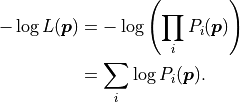
However, usually parameter estimation is not performed by using the likelihood, but by using its negative logarithm, the so-called negative log-likelihood:

$- \log L(\bm{p}) &= -\log \left( \prod_i P_i(\bm{p}) \right) \\ &= \sum_i \log P_i(\bm{p}).$

This transformation is allowed because logarithms are strictly monotonically increasing functions, and therefore the negative logarithm of any function will have its global minimum at the same place where the likelihood is maximal. The parameter values $\bm{p}$ that minimize the negative log-likelihood will therefore also maximize the likelihood.

While the above transformation may seem nonsensical at first, there are important advantages to calculating the negative log-likelihood over the likelihood:

The product of the probabilities $\prod_i P_i$ is replaced by a sum over the logarithms of the probabilities $\sum_i \log P_i$ . This is a numerical advantage because sums can be calculated much more quickly than products, and sums are numerically more stable than products of many small numbers.
Because the probabilities $P_i$ are oftentimes proportional to exponential functions, calculating their logarithm is actually faster because it reduces the number of necessary operations.
Taking the negative logarithm allows for always using the same numerical optimizers to minimize different cost functions.

As an example, let us look at the negative log-likelihood of data with uncertainties that assume a normal distribution:

$-\log \prod_i P_i(\bm{p}) & = - \log \prod_i \frac{1}{\sqrt[]{2 \pi} \: \sigma_i} \exp\left( \frac{1}{2} \left( \frac{d_i - m_i(\bm{p})}{\sigma_i} \right)^2\right) \\ & = - \sum_i \log \frac{1}{\sqrt[]{2 \pi} \: \sigma_i} + \sum_i \frac{1}{2} \left( \frac{d_i - m_i(\bm{p})}{\sigma_i} \right)^2 \\ & = - \log L_\mathrm{max} + \frac{1}{2} \chi^2$

As we can see the logarithm cancels out the exponential function of the normal distribution and we are left with two parts:

The first is a constant part that is represented by $-\log L_\mathrm{max}$ . This is the minimum value the neg log-likelihood could possibly take on if the model $\bm{m}$ were to exactly fit the data $\bm{d}$ .

The second part can be summed up as $\frac{1}{2} \chi^2$ . As it turns the method of least squares is a special case of the method of maximum likelihood where all data points have normally distributed uncertainties.

Handling uncertainties¶

Standard cost functions treat fit data as a series of measurements in the y direction and can directly make use of the corresponding uncertainties in the y direction. Unfortunately uncertainties in the x direction cannot be used directly. However, x uncertainties can be turned into y uncertainties by multiplying them with the derivative of the model function to project them onto the y axis; this is what kafe2 does. The xy covariance matrix is then calculated as follows:

$\bm{V}_{ij} = \bm{V}_{y,ij} + f'\left(x_i\right)f'\left(x_j\right)\bm{V}_{x,ij}.$

Warning

This procedure is only accurate if the model function is approximately linear on the scale of the x uncertainties.

Other types of uncertainties¶

As the statistical uncertainty for histograms is a Poisson distribution for the number of entries in each bin, a negative log-likelihood cost function with a Poisson probability can be used, where ${\bf d}$ are the measurements or data points and ${\bf m}$ are the model predictions:

$C = -2 \ln \prod_j \frac{{m_j}^{d_j}}{d_j!}\exp(-m_j).$

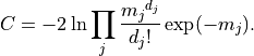
As the variance of a Poisson distribution is equal to the mean value, no uncertainties have to be given when using Poisson uncertainties.

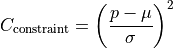
Parameter constraints¶

When performing a fit, some values of the model function might have already been determined in previous experiments. Those results and uncertainties can then be used to constrain the given parameters in a new fit. This eliminates the need to manually propagate the uncertainties on the final fit results, as it’s now done numerically.

Parameter constraints are taken into account during the parameter estimation by adding an extra penalty to the cost function. The value of the penalty is determined by how well the parameter lies within its constraints. With the cost functions used above $C \equiv C_0$ , the new cost function then reads as

$C_\mathrm{total} = C_0 + C_\mathrm{constraint}$

In general the penalty is given by the current parameter values $\bm{p}$ , the expected parameter values $\bm{\mu}$ and the covariance matrix $V$ describing the values and correlations between the constraints on the parameters:

$C_\mathrm{constraint} = (\bm{p} - \bm{\mu})^T V^{-1} (\bm{p} - \bm{\mu})$

For a single parameter this simplifies to:

$C_\mathrm{constraint} = \left ( \frac{p-\mu}{\sigma} \right )^2$