Hidden Sector Decay Spectrometer (HSDS)
The Hidden Sector Decay Spectrometer (HSDS) is the largest component, contributing most to the total length of \(100\,\text{m}\) - \(120\,\text{m}\) of the SHiP experiment. It is designed to enable the decay of long-lived, weakly interacting particles in flight and to detect their decay products. The HSDS is located downstream of the muon shield and consists of a 50 m long helium filled decay volume surrounded by Surround Background Taggers and a subsequent Spectrometer.
Decay-Volume
The decay volume is a wedge-shaped \(50\,\text{m}\) long helium filled volume. A schematic overview of the decay volume is shown in Fig. 1. Helium was chosen as the filling gas because it is an inert atomic gas with a low atomic number (Z), which suppresses Standard Model interactions and thus the production of secondary particles. These secondary particles would otherwise contribute to the background. Instead, SHiP aims to reduce the background to a minimum, aiming for a "zero background" environment. Within the \(50\,\text{m}\) long decay volume, long-lived particles are expected to decay in flight. Their decay products are then detected by the spectrometer following the decay volume.
Within the HSDS, the following non-SM2 particles are expected:
- Dark photons
- Axions and Axion-like particles
- Heavy neutron leptons
- Other long-lived particles predicted by extensions of the Standard Model
All of them are possible candidates for dark matter and are expected to decay into Standard Model particles within the decay volume. These SM-particles should not interact within the decay volume and survive the flight to the spectrometer instead, where they are detected. The signal of the detector is going to be a displaced vertex, which is a point in space where the decay products of the non-SM particle originate from. The interaction point is expected to be located within the HSDS decay volume and not within the muon shield or the scattering and neutrino detector.
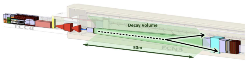
Fig. 1: Schematic of the SHiP experiment, highlighting the \(50\,\text{m}\) long decay volume within the HSDS.6
Shape of the Decay Volume
The current geometry of the decay volume is set to be a \(50\,\text{m}\) long wedge-shape. The size of the entrance and exit area is not yet finalized, but recent designs suggest a size of \(1\,\text{m}\) length and \(2.7\,\text{m}\) height at the upstream end and a size of \(4\,\text{m}\) to \(6\,\text{m}\) length and \(6\,\text{m}\) to \(8\,\text{m}\) height at the downstream end45. The length was determined by maximising the probability for a decay to occur within the detector while still keeping the size small enough to build it. For \(N_0\) particles with lifetime \(\tau\) the decay rate is given by the formula:
This yields the probability for a particle to decay within a time interval \(T\) as
The decay length \(L\) of a particle is defined as the distance it travels before decaying. It is given by the formula:
with the speed of light \(c\), the lifetime of the particle \(\tau_0\), the \(\beta\) factor \(\beta = \frac{v}{c} \approx 1\) and the Lorentz factor \(\gamma = \frac{1}{\sqrt{1 - \beta^2}}\) to account for the time dilation due to the relativistic speed of the particle. The lifetime \(\tau\) can be expressed as
with the decay width \(\Gamma\) of the particle. For Long-lived particles (LLP) the decay width is very small, because the interaction of the particle with the Standard Model is very weak. This results in a long lifetime \(\tau\) and thus a long decay length \(L\).
With this, the probability for a particle to decay within a distance \(x\) can be expressed as:
where \(x\) is the distance from the production point of the particle to the entrance of the decay volume and \(\Delta{}x\) is the length of the decay volume (the infamous \(50\,\text{m}\)). Equation \(\eqref{equ-decay-volume}\) shows that the probability for a particle to decay within the decay volume grows with the length \(\Delta{}x\), up to the limit of \(P = 1 - e^{-x/L}\) for \(\Delta{}x \to \infty\). Since the probability follows an exponential decay, the probability reaches a limit where the increase of the decay volume length does not significantly increase the probability for a particle to decay within the volume.
When the decay occurs, the products are expected to be Standard Model particles, which also have a certain lifetime and decay length. The design of the vessel should ensure that these decay products can sill reach the detector spectrometer. Typical expected decay products for Heavy Neutral Leptons (\(N\)) are:
And for Dark Photons (\(A'\)) or Axion-like particles (\(a\)):
The electrons, photons and positrons (in vacuum) are stable. The lifetimes of the other decay products need to be long enough to reach the spectrometer, which should be considered when designing the decay volume.
To find an optimal length for the decay volume, the probability in equation \(\eqref{equ-decay-volume}\) was combined with the number of produced particles \(N_\text{prod}\) and the reconstruction acceptance \(\epsilon_\text{reco}\) to yield the number of expected signals within the decay volume7:
The reconstruction acceptance \(\epsilon_\text{reco}\) contains many factors, such as:
- The geometrical acceptance of the detector, which is the probability for the decay products to reach the detector active volume.
- The reconstruction efficiency, which describes the probability that the tracks of the charged decay product are reconstructed properly.
- The identification efficiencym accounting for the probability that the tracks of the decay products are identified correctly as the expected particle type, e.g. muons, electrons, pions, etc.
- The trigger efficiency of the detector, which is the probability for a signal to trigger the detector and be recorded.
- The selection efficiency of the analysis, accounting for the fact that a recorded signal has to pass the offline analysis requirements.
- The survival probability of the decay products on their way to the detector, accounting for losses due to secondary decays or interactions within the vessel.
Using the FairShip simulation framework, which combines different simulation tools such as Pythia8, FLUKA and Geant4, the number of expected signals \(N_\text{signal}\) was calculated for different decay volume lengths \(\Delta{x}\). The Analysis and simulation chain for the optimization is described in the Simulation section.
The number of expected signals \(N_\text{signal}\) was calculated for different decay volume lengths \(\Delta{x}\). The acceptance of the SHiP experiment for different decay volume lengths \(\Delta{x}\) is shown in Fig. 2. The plot shows, that the acceptance saturates for \(\Delta{x} \gtrsim 50\,\text{m}\), which is why the decay volume was chosen to be \(50\,\text{m}\) long8.
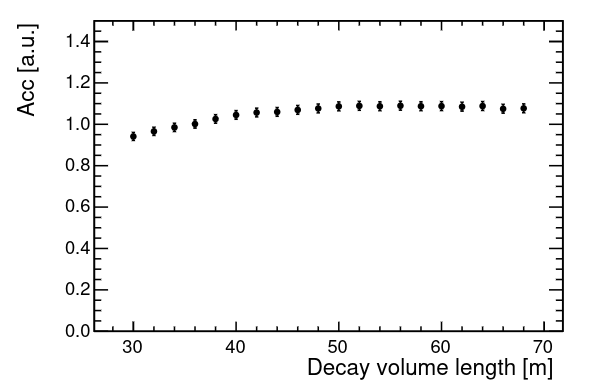
Fig. 2: Acceptance of the SHiP experiment for different decay volume lengths \(\Delta{x}\). The acceptance saturates for \(\Delta{x} \gtrsim 50\,\text{m}\), which is why the decay volume was chosen to be \(50\,\text{m}\) long.8
Since the cross section of the vessel was not defined at the time of simulation, a \(5\,\text{m} \times 10\,\text{m}\) elliptical cylinder was chosen for the simulation.
Design choices for Helium
Earlier design had kept the decay volume under a vacuum1 at \(10^{-2}\,\text{bar}\) with a total vacuum volume of \(\approx 2040\,\text{m}^3\). This was changed to helium under atmospheric pressure in order to reduce the cost and complexity of the experiment. Furthermore, the Vacuum approach would have required a thicker vessel wall to provide the appropriate stability for a vacuum container this size (which would start to bend), which would have reduced the detector acceptance and required the detector (tracker and spectrometer magnet) to be placed within the vacuum, since it would have not been acceptable to place a large amount of material in front of the detector. This is a common problem in the design of detectors: The ideal particle detector would have no material to reduce the interaction of particles while simultaneously cover everything in order to detect all particles as precise as possible. In practice, this is not possible and compromises have to be made.
By using helium, which is a gas with a density of \(\rho_\text{He} = 0.1786\,\frac{\text{kg}}{\text{m}^3}\) (at \(1\,\text{bar}\) pressure and \(0^\circ\text{C}\) temperature)3, the vessel wall can be made thinner than in the original plan14, which increases the acceptance of the detector. The low atomic number of \(\text{Z} = 2\) for helium also yields a low probability for SM interactions for High Energy Particles as well as a low probability for scattering of the decay products within the vessel. A comparison between these two approaches is summarized in Table 1.
Tab. 1: Comparison of the two approaches for the decay volume: Vacuum vs. Helium. The helium approach is preferred due to its low cost and easy construction, while still providing a low probability for SM interactions within the vessel.
| Vacuum | Helium |
|---|---|
| nearly no SM interactions within the vessel | low probability for SM interactions within the vessel |
| very heavy and thick vessel walls | light and thin vessel walls |
| high requirements for the vessel stability and tightness | very easy construction |
Surround Background Tagger (SBT)
To reduce the background form cosmic neutrinos or muon interactions within the vessel, the walls of the decay volume are completely surrounded by a Surround Background Tagger (SBT). Neutrinos could interact with the gas molecules inside the vessel and produce secondary particles, which result in background events triggering the detector and imitating the signal of a decay vertex originating from the inside of the vessel. These type of background signals can also be caused in the same way by muons. Since the number of background interactions is proportional to the density of the vessel volume, a vacuum vessel was chosen in the initial approach for the HSDS. The reasons why this design was replaced by a helium filled vessel are explained in the Helium-filled Gas Volume section.
The vessel is surrounded by scintillator panels910 to detect charged particles entering the vessel through the walls apart from the upstream and downstream ends. These taggers identify neutrino- and muon-induced interactions with the vessel walls, which may produce neutral long-lived secondary particles, decaying inside the vessel and mimicking the signal events in the spectrometer. Whenever an event is registered in the SBT, the event is tagged as a background event and rejected from the analysis. Therefore, a veto efficiency, defined as the ratio of accepted events to total events, is used to quantify the performance of the SBT:
For SHiP this veto efficiency is required to be very high, because the expected number of signal events is very low and the experiment aims for a "zero background" environment.
Upstream Background Tagger (UBT)
Similarly to the SBT an "Upstream Background Tagger" (UBT) is used to detect background events from the upstream region. Within the vessel, the hidden particle is invisible. The measurement of the spectrometer resolves the tracks of the decay products and allows to reconstruct the decay vertex. A problem arises when particles from the upstream region enter the vessel. Possible candidates for this are excess-muons that were not deflected by the muon shield or other particles produced in the target or the scattering and neutrino detector. To mitigate this, the UBT is placed upstream of the vessel to detect these particles and tag them as background events, as depicted in the following diagram:
flowchart TD

    A["Proton Beam"]
    B["Target"]
    C["Active Myon shield"]
    D["Upstream Background Tagger (UBT)"]
    E["Decay Volume"]
    F["Spectrometer"]

    A --> B
    B --> C
    C --> D
    D --> E
    E --> F
Similar to the SBT, an event is excluded from the analysis if it is registered in the UBT. The veto efficiency of the UBT is defined in the same way as for the SBT, as shown in equation \(\eqref{equ-veto-efficiency}\).
Warning
The "Upstream Background Tagger" is not the same as the "Scattering & Neutrino Detector", even though they are both located upstream of the decay volume and both deal with the background rejection. The UBT is part of the HSDS and used to suppress background events from the upstream region. The SND is a separate detector, planed to be used for neutrino physics measurements. Some SHiP Documents do not describe this difference clearly, which can lead to confusion. The SND and the HSDS are separate components.
Downstream Spectrometer
The downstream spectrometer, often called "HS Spectrometer", is used to detect decay products from possible "Hidden particle" decays within the decay volume. A location of the spectrometer can be seen in Fig. 3.
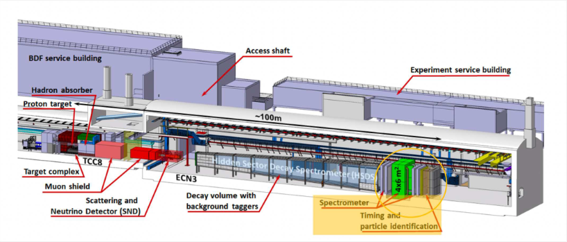
Fig. 3: Schematic of the SHiP experiment, highlighting the downstream spectrometer within the HSDS.11
This section describes the components of the spectrometer based on the newest design considerations, where the HS has a total width of \(4\,\text{m}\) and a height of \(6\,\text{m}\) at the downstream end of the decay volume. The description might differ from other documents, relating to the fact that the design of the SHiP experiment is still in progress and not finalized yet. The order of the components of the HS Spectrometer are visualised in the following diagram:
flowchart TB

    %% Beam direction
    DV[["Decay Volume"]]
    DV ==> T1
    subgraph "  "
    T1["Straw Tracker T1"]
    T1 --> T2
    T2["Straw Tracker T2"]
    end
    T2 --> MAG
    MAG["Dipole Magnet"]
    MAG --> T3
    subgraph " "
    T3["Straw Tracker T3"]
    T3 --> T4
    T4["Straw Tracker T4"]
    end
    T4 --> Timing
    Timing["High Precision Timing Detector"]
    Timing --> ECAL
    ECAL["Electromagnetic Calorimeter"]
    ECAL --> HCAL
    HCAL["Hadronic Calorimeter"]
    HCAL --> Muon
    Muon["Muon Identification System"]
The subsequent sections describe the components of the spectrometer in more detail.
Tracker and Magnet
Within the HS Spectrometer, \(2 \times 2\) stations of "straw tube trackers" (STT) are used to measure the tracks of charged particles and reconstruct the vertices. Two of them are placed before the magnet and two after the magnet. The magnet is a superconducting dipole magnet to bend the tracks of charged particles and measure their momentum. It has a field strength peaking around \(0.5\,\text{T}\) and a field integral of \(\int B \dd L = 0.65\,\text{Tm}\) (the total magnetic strength experienced by a particle moving along a path). Charged particles are deflected by the magnetic field, which allows to measure their momentum based on the curvature of their tracks.
The STT are used to measure the position of charged particles and reconstruct their tracks. The are build from Cu/Au-coated Mylar drift tubes, which are arranged in layers. The design choices for the STT are based on the NA62 experiment1, which used a similar design. Small tubes are cheaper to produce for large areas and have a low material budget, which reduces the probability for interactions of multiple scattering of the particles within the detector.
Each STT module consists of 4 double layers of drift tubes, which are arranged in different orientations each, to allow for a 2D reconstruction of the intersection point of the tracks with the STT. The layers are rotated by the angles \(0^\circ\), \(+5^\circ\), \(-5^\circ\) and \(90^\circ\). The following diagram sums the design of a single STT module up:
flowchart TB

    T["One Straw Tracker Station"]

    T --> V1["View X"]
    T --> V2["View U<br>(+5°)"]
    T --> V3["View V<br>(-5°)"]
    T --> V4["View Y"]

    V1 --> Straw1["2 Straw Layers"]
    V2 --> Straw2["2 Straw Layers"]
    V3 --> Straw3["2 Straw Layers"]
    V4 --> Straw4["2 Straw Layers"]
Each STT module contains 8 layers in total. The hit efficiency of the STT is expected to be \(\gt 99\%\). The modules 1 and 2, which are placed before the magnet, are used to reconstruct the initial movement of the incident charged particle before the magnetic field deflects it. Afterwarts, the layers 3 and 4 reconstruct the deflection and allow to measure its momentum. In total, a ST modules contains \(\approx 10000\) channels.
From the bending angle \(\Theta\) of the deflected track, the impulse \(p\) of the particle can be calculated using the formula:
High-Precision Timing Detector (HPTD)
SHiP works with an intensely high number of protons on its target. This results in a high number of particles produced in the target, which can lead to multiple tracks being measured at nearly the same time in the tracker. As an example the following situation is considered: Two independent muons are measured in the tracker at nearly the same time, both of which can be reconstructed to the same vertex within the decay volume. The question arises, whether these two muons originate from the same decay vertex or if they are two independent muons that just happen to be measured at nearly the same time and reconstructed to the same vertex. To resolve this ambiguity, a High-Precision Timing Detector (HPTD) is used to measure the arrival time of the particles with a precision of \(\approx 100\,\text{ps}\). Particles from the same decay vertex are expected to arrive at the HPTD at nearly the same time, while independent particles are expected to arrive at different times.
With a timing precision of \(\Delta{}t \approx 100\,\text{ps}\), the HPTD is able to resolve particles that are separated by a distance of \(\Delta{}x = c \cdot \Delta{}t \approx 3 \cdot 10^8\,\frac{\text{m}}{\text{s}} \cdot 100 \cdot 10^{-12}\,\text{s} = 3\,\text{cm}\) at the speed of light.
For the structure of the HTPD, a scintillator-based design is planed12. The HPTD is separated in 3 columns with a height of \(8\,\text{m}\), overlapping each other at around \(5\,\text{mm}\). Each column contains 111 rows of scintillator bars of \(135\,\text{cm}\) width, \(6\,\text{cm}\) height and \(1\,\text{cm}\) thickness. At both ends of the bar, Silocon Photomultipliers (SiPM) are used to detect the scintillation light and convert it into an electrical signal. In total, this design yields \(666\) channels for the HPTD. From the arrival time on the left and right SiPM (\(t_\text{left}, t_\text{right}\)) of a bar, the incident position of the particle can be calculated to:
where \(c\) refers to the speed of light in the scintillator material.
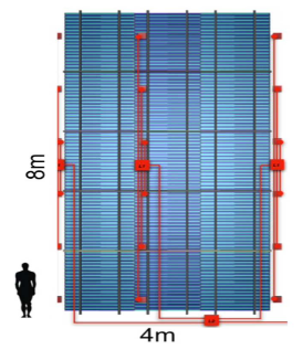
Fig. 4: A CAD model of the High-Precision Timing Detector (HPTD) within the HSDS. The HPTD is separated into 3 columns with a small overlap.12
Calorimeter and Muon System
The final components of the HS Spectrometer are a Electromagnetic Calorimeter (ECal), a Hadronic Calorimeter (HCal) and a Muon Identification System. The ECal is used to measure the energy of electrons and photons, while the HCal is used to measure the energy of hadrons. Afterwards, a Muon Identification System is used to reliably distinguish muons from pions.
The ECal is a sampling calorimeter, consisting of 40 layers of iron absorbers at the length of \(\frac{1}{20}\lambda\) each with plastic scintillators in between them. It measures a total length of \(74.8\,\text{cm}\). Electromagnetic Showers are expected to be reconstructed with a resolution \(\lt 5\,\text{mrad}\). The HCal uses 5 layers of iron absorbers at the length of \(1\lambda\) each with plastic scintillators in between them, at a total length of \(88\,\text{cm}\). In total, the calorimeter measures 7 nuclear interaction lengths.
The HCal absorbs most of the hadronic showers before they can reach the muon identification system. The muon system is a sampling calorimeter, consisting of 4 active stations, \(6\,\text{m}\) wide and \(12\,\text{m}\) high with iron filter plates in between them. Each layer contains \(3200\) scintillator tiles (\(12800\) channels in total) to detect the muons. With a time resolution \(\lt 300\,\text{ps}\) the muon system allows for a 2D coordinate reconstruction of the track incident on each layer13. Fig. 5 shows a CAD model of the SHiP experiment, highlighting the downstream spectrometer and its components within the HSDS.
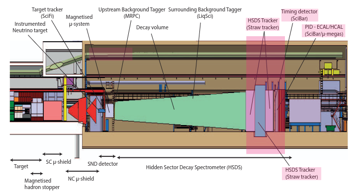
Fig. 5: A CAD Drawing of the SHiP experiment, highlighting the downstream spectrometer within the HSDS.12 The description "HSDS Tracker (Straw Tracker)" on the lower right is falsely labeled and should be referencing the "Deflection Magnet".
A Collection of Corporate Bullshit Terms
Within the SHiP Documents a lot of terms are used interchangeably, which leads to confusion. The following list summarizes some of them and clarifies their meaning:
- "SciBar": Originally, this term was the name of a standalone detector module but now it is used as an abbreviation for "Scintillator Bars" and describes a technology used in the SBT, UBT, HPDT, ECal, HCal and Muon System. A SciBar system uses bar-shaped scintillators with optic fibers running through them. Both ends are attached to SiPMs to measure the scintillation light. From the arrival times of the light on both ends \(t_1\) and \(t_2\), the incident position of the particle can be calculated to \(x_\text{incidence} = \frac{c}{2} (t_1 - t_2)\), where \(c\) is the speed of light in the scintillator material. Compared to a single scintillator tile, a SciBar system allows for a cheaper construction while still maintaining a good enough spatial resolution.
- "µ-megas": This name stand for "Micro-MEsh GAseous Structure" and is often written as "Micromegas". It describes a type of "micro-pattern gaseous detector" (MPGD), which is made out of two gas-filled chambers separated by a very thin metallic mesh. The first region (drift region) applies an electric field between the upstream entrance of the particles and the mesh, causing the ionization of gas molecules and the drift of electrons towards the mesh. The second, very small region (amplification gap), applies a much stronger electric field between the mesh and the readout plane, causing an avalanche-like amplification of the electrons. In some SHiP Designs Micromegas were proposed as the active readout for the Myon system within the HSDS, being replaced by the SciBar design in the newest design considerations.
- "LiqSci" is short for "Liquid Scintillator". In the initial approach, the vacuum vessel was in a bath of liquid scintillator material to implement the SBC. After the replacement of the vacuum vessel by a helium-filled vessel, this detail was not discussed any further and left open. It is unclear whether the SBC is still planed to be implemented in a bath of liquid scintillator or if it is planed to use another approach.
- "MRPC" stands for "Multi-gap Resistive Plate Chamber" and should have been used as the active component for the UBT. The design is close to a Micromegas, but uses more than two chambers to amplify the ionization electrons and produce multiple avalanches simultaneously. The readout electrodes are covering the set of chambers on both ends and measure the arrival time and a spatial resolution of the incident particle. It is unclear, weather an MRPC or a SciBar system is planed to be used for the UBT.
-
https://cds.cern.ch/record/2704147/files/SPSC-SR-263.pdf, Section 3.5 ↩↩
-
https://agenda.infn.it/event/43758/contributions/253051/attachments/134295/200895/SHiP_LDMA_2025.pdf, Slide 11 ↩
-
https://www.imperial.ac.uk/news/252333/imperial-scientists-lead-search-hidden-particles/ ↩
-
Source: https://agenda.infn.it/event/43758/contributions/253051/attachments/134295/200895/SHiP_LDMA_2025.pdf, Slide 11, with own modifications. ↩
-
https://discovery.ucl.ac.uk/id/eprint/10073757/7/Campanelli_Sensitivity%20of%20the%20SHiP%20experiment%20to%20Heavy%20Neutral%20Leptons_VoR.pdf, Equation (4.6) ↩
-
https://arxiv.org/pdf/1504.04956, Section 2, Figure 2.4 ↩↩
-
https://cds.cern.ch/record/2704147/files/SPSC-SR-263.pdf, Section 3.5 ↩
-
https://arxiv.org/pdf/1504.04956, Section 4.5 ↩
-
Source: https://agenda.infn.it/event/43758/contributions/253051/attachments/134295/200895/SHiP_LDMA_2025.pdf, Slide 13 ↩
-
Source: https://agenda.infn.it/event/43758/contributions/253051/attachments/134295/200895/SHiP_LDMA_2025.pdf, Slide 15 ↩↩↩
-
https://cds.cern.ch/record/2704147/files/SPSC-SR-263.pdf, Section 3.14 ↩
-
https://doi.org/10.1007/s43452-020-00152-9, Page 3 ff. ↩